As an application developer, you must give some thought to your choice of database best suited for your needs since you are not going to implement your storage engine from scratch. In order to make the choice, you should at least have a rough idea of how each database works under the hood. In this article we are diving into the two families of storage engines: ***Log-Structured (LSM)***and Page-Oriented(B-trees).

Data Structures That Power Databases

Many databases internally use a log which is an append-only data file. The word log is generally used to refer to application logs, where the app outputs what's happening. Here, the log is used in a more general sense: an append-only sequence of records. It doesn't have to be human-readable; it might be binary. Real databases have many issues dealing with log files (such as concurrency control, reclaiming disk space).

On the other hand, if you want to search for a key, you've to scan the entire database file from beginning to end (O(n)). If you double the records in your database, the search takes twice as long. That's not good.

To efficiently find the key in the database, we need a different data structure: an index. An index is an additional structure that is derived from the primary data. Many DBs allow you to add and remove indexes, which affects the performance of the queries. Maintaining additional structures incurs overhead, especially on writes. Any kind of index usually slows down writes, because the index needs to be updated every time data is written.

There is an important trade-off in storage systems: well-chosen indexes speed up reads but every index slows down writes. For this reason, DBs don't usually index everything by default but require you, the application developer to do the same.

Hash Indexes

Let’s start with indexes for key-value data. This is not the only kind of data you can index, but it’s very common, and it’s a useful building block for more complex indexes.

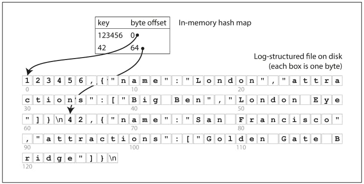
The simplest possible indexing strategy is this: keep an in-memory hash map where every key is mapped to a byte offset in the data file-the location at which the value can be found, as illustrated in the following figure. Whenever you append a new key-value pair to the file, you also update the hash map (this works for both insertion and updation of keys). When you want to look up a value, use the hash map to find the offset in the data file, seek that location, and read the value. This is simplistic, but the *BitCask (*storage engine in Riak) does this underneath the hood.

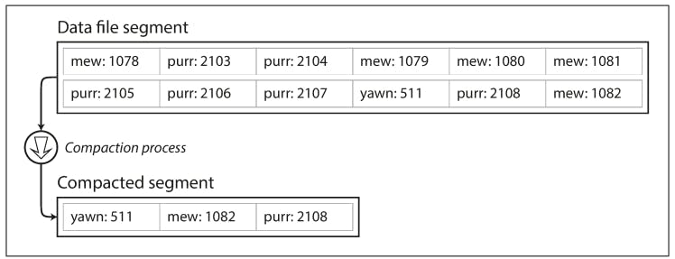
As described so far, we are only ever appending to a file-so how do we avoid eventually running out of disk space? A good solution is to maintain segments of a certain size and making subsequent writes to a new segment file. We can then perform compaction on these segments, as below. Compaction means throwing away duplicate keys in the log and keeping only the most recent update for each key.

SSTables and LSM-Trees

In the previous figure, we had a log-structured storage segment which is a sequence of key-value pairs. Now we can make a simple change to the format of our segment files: we require that the sequence of key-value pairs is sorted by key. At first glance, that requirement seems to break our ability to use sequential writes, but we’ll get to that in a moment. We call this format Sorted String Table, or SSTable. We also require that each key only appears once within each merged segment file (the compaction process already ensures that). SSTables have several big advantages over log segments with hash indexes:

1. Merging: segments is simple and efficient, even if the files are bigger than the available memory. The approach is like the one used in the mergesort algorithm.

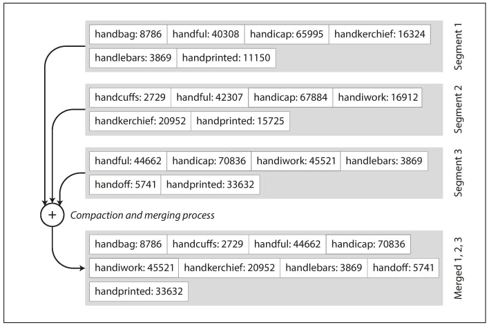
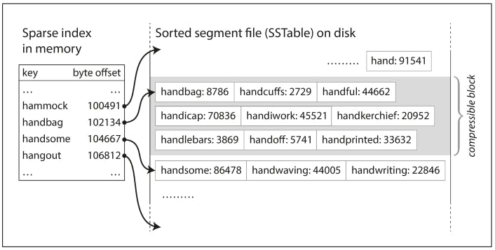
To find particular key, you no longer need to keep an index of all the keys in memory. Say you’re looking for the key handiwork, but you don’t know the exact offset of that key. However, you do know the offsets for the keys handbag and handsome. This means you can jump to the offset for handbag and scan from there until you find handiwork (or not, if the key is not present in the file).

Constructing and Maintaining SSTables

Fine, you've built SSTables, but how to sort the data based on the keys in the first place? Incoming writes can occur in any order.

Maintaining a sorted structure on disk is possible , but in memory is much easier. There are many tree data structures that you can use, such as red-black trees or AVL trees. With these data structures, you can insert keys in any order and read them back in sorted order. We can now make our storage engine work as follows:

• Upon a write, add it to an in-memory balanced tree data structure. This in-memory tree is sometimes called a memtable.

• When the memtable gets bigger than some threshold-typically a few megabytes —write it out to disk as an SSTable file. The new SSTable file becomes the most recent segment of the database. While the SSTable is being written out to disk, writes can continue to a new memtable instance.

• In order to serve a read request, first try to find the key in the memtable, then in the most recent on-disk segment, then in the next-older segment, etc.

• From time to time, run a merging and compaction process in the background.

Making LSM-Trees out of SSTables

Originally this indexing structure was described under the name Log-Structured Merge-Tree (or LSM-Tree), building on earlier work on log-structured filesystems. Similar storage engine is used in Cassandra and HBase, both of which were inspired by Google’s Bigtable paper (which introduced the terms SSTable and memtable).

Even though there are many subtleties, the basic idea of LSM-trees - keeping a cascade of SSTables that are merged in the background - is simple and effective. Even when the dataset is much bigger than the available memory it continues to work well. Since data is stored in sorted order, you can efficiently perform range queries (scanning all keys above some minimum and up to some maximum), and because the disk writes are sequential the LSM-tree can support remarkably high write throughput.

B-Trees

The log-structured indexes we have discussed so far are gaining acceptance, but they are not the most common type of index. The most widely used indexing structure is quite different: the B-tree.

Like SSTables, B-trees keep key-value pairs sorted by key, which allows efficient key-value lookups and range queries. But that’s where the similarity ends: B-trees have a very different design philosophy.

The log-structured indexes we saw earlier break the database down into variable-size segments, typically several megabytes or more in size, and always write a segment sequentially. By contrast, B-trees break the database down into fixed-size blocks, traditionally 4 KB in size (sometimes bigger), and read or write one page at a time. This design corresponds more closely to the underlying hardware, as disks are also arranged in fixed-size blocks.

Each page can be identified using an address or location, which allows one page to refer to another - similar to a pointer, but on disk instead of in memory. We can use these page references to construct a tree of pages as follows:

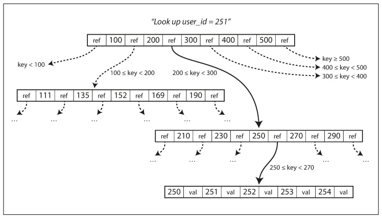
In the above figure, we are looking for key 251, so we know that we need to follow the page reference between the boundaries 200 and 300. That takes us to a similar-looking page that further breaks down the 200–300 range into subranges. Eventually, we get down to a page containing individual keys (a leaf page), which either contains the value for each key inline or contains references to the pages where the values can be found.

The number of references to child pages in one page of the B-tree is called the branching factor. For example, in the above figure, the branching factor is six. In practice, the branching factor depends on the amount of space required to store the page references and the range boundaries, but typically it is several hundred.

It is ensured that the tree remains balanced: a B-tree with n keys always has a depth of O(log n). Most databases can fit into a B-tree that is three or four levels deep, so you don’t need to follow many page references to find the page you are looking for (A four-level tree of 4 KB pages with a branching factor of 500 can store up to 256 TB).

To learn more about B-Trees and B+, B* trees, go through this textbook: here

Comparing LSM-Trees and B-trees

Even though B-trees are generally more mature than LSM-tree, LSM-trees are also interesting due to their performance characteristics. As a rule of thumb, LSM-trees are typically faster for writes, whereas B-trees are thought to be faster for reads. Reads are typically slower on LSM-trees because they have to check several different data structures and SSTables at different stages of compaction.

However, benchmarks are often inconclusive and sensitive to details of the workload. You need to test systems with your particular workload in order to make a valid comparison.

If you have any queries, please comment below.

References

1. Designing Data-Intensive Applications: The Big Ideas Behind Reliable, Scalable, and Maintainable Systems - Martin Kleppmann

2. File Structures: An Object-Oriented Approach with C++ - Michael J Folk, Bill Zoellick, Greg Riccardi